Noise cutoff (noise_cutoff)
Calculation
Metric describing whether an amplitude distribution is cut off as it approaches zero, similar to amplitude cutoff but without a Gaussian assumption.
The noise cutoff metric assesses whether a unit’s spike‐amplitude distribution is truncated at the low-end, which may be due to the high amplitude detection threshold in the deconvolution step, i.e., if low‐amplitude spikes were missed. It does not assume a Gaussian shape; instead, it directly compares counts in the low‐amplitude bins to counts in high‐amplitude bins.
Build a histogram
For each unit, divide all amplitudes into
n_binsequally spaced bins over the range of the amplitude. If the number of spikes is large, you may consider using a largern_bins. For a small number of spikes, consider a smallern_bins. Let \(n_i\) denote the count in the \(i\)-th bin.- Identify the “low” region
Compute the amplitude value at the specified
low_quantile(for example, 0.10 = 10th percentile), denoted as \(\text{amp}_{low}\).Find all histogram bins whose upper edge is below that quantile value. These bins form the “low‐quantile region”.
Compute
\[L_{\mathrm{bins}} = \bigl\{i : \text{upper_edge}_i \le \text{amp}_{low}\bigr\}, \quad \mu_{\mathrm{low}} = \frac{1}{|L_{\mathrm{bins}}|}\sum_{i\in L_{\mathrm{bins}}} n_i.\]
Identify the “high” region
Compute the amplitude value at the specified
high_quantile(for example, 0.25 = top 25th percentile), denoted as \(\text{amp}_{high}\).Find all histogram bins whose lower edge is greater than that quantile value. These bins form the “high‐quantile region”.
Compute
\[\begin{split}H_{\mathrm{bins}} &= \bigl\{i : \text{lower_edge}_i \ge \text{amp}_{high}\bigr\}, \\ \mu_{\mathrm{high}} &= \frac{1}{|H_{\mathrm{bins}}|}\sum_{i\in H_{\mathrm{bins}}} n_i, \quad \sigma_{\mathrm{high}} = \sqrt{\frac{1}{|H_{\mathrm{bins}}|-1}\sum_{i\in H_{\mathrm{bins}}}\bigl(n_i-\mu_{\mathrm{high}} \bigr)^2}.\end{split}\]Compute cutoff
The cutoff is given by how many standard deviations away the low-amplitude bins are from the high-amplitude bins, defined as
\[\mathrm{cutoff} = \frac{\mu_{\mathrm{low}} - \mu_{\mathrm{high}}}{\sigma_{\mathrm{high}}}.\]If no low‐quantile bins exist, a warning is issued and
cutoff = NaN.If no high‐quantile bins exist or \(\sigma_{\mathrm{high}} = 0\), a warning is issued and
cutoff = NaN.
Compute the low-to-peak ratio
Let \(M = \max_i\,n_i\) be the height of the largest bin in the histogram.
Define
\[\mathrm{ratio} = \frac{\mu_{\mathrm{low}}}{M}.\]If there are no low bins, \(\mathrm{ratio} = NaN\).
Together, (cutoff, ratio) quantify how suppressed the low‐end of the amplitude distribution is relative to the top quantile and to the peak.
Expectation and use
Noise cutoff attempts to describe whether an amplitude distribution is cut off.
Larger values of cutoff and ratio suggest that the distribution is cut-off.
IBL uses the default value of 1 (equivalent to e.g. low_quantile=0.01, n_bins=100) to choose the number of
lower bins, with a suggested threshold of 5 for cutoff to determine whether a unit is cut off or not.
In practice, the IBL threshold is quite conservative, and a lower threshold might work better for your data.
We suggest plotting the data using the plot_amplitudes() widget to view your data when choosing your threshold.
It is suggested to use this metric when the amplitude histogram is unimodal.
The metric is loosely based on [Hill]’s amplitude cutoff, but is here adapted (originally by [IBL2024]) to avoid making the Gaussian assumption on spike distributions.
Example code
import numpy as np
import matplotlib.pyplot as plt
from spikeinterface.full as si

# Suppose `sorting_analyzer` has been computed with spike amplitudes:
# Select units you are interested in visualizing
unit_ids = ...

# Compute noise_cutoff:
summary_dict = compute_noise_cutoffs(
    sorting_analyzer=sorting_analyzer
    high_quantile=0.25,
    low_quantile=0.10,
    n_bins=100,
    unit_ids=unit_ids
)
Reference
- spikeinterface.qualitymetrics.misc_metrics.compute_noise_cutoffs(sorting_analyzer, high_quantile=0.25, low_quantile=0.1, n_bins=100, unit_ids=None)
A metric to determine if a unit’s amplitude distribution is cut off as it approaches zero, without assuming a Gaussian distribution.
Based on the histogram of the (transformed) amplitude:
1. This method compares counts in the lower-amplitude bins to counts in the top ‘high_quantile’ of the amplitude range. It computes the mean and std of an upper quantile of the distribution, and calculates how many standard deviations away from that mean the lower-quantile bins lie.
The method also compares the counts in the lower-amplitude bins to the count in the highest bin and return their ratio.
- Parameters:
- sorting_analyzerSortingAnalyzer
A SortingAnalyzer object.
- high_quantilefloat, default: 0.25
Quantile of the amplitude range above which values are treated as “high” (e.g. 0.25 = top 25%), the reference region.
- low_quantileint, default: 0.1
Quantile of the amplitude range below which values are treated as “low” (e.g. 0.1 = lower 10%), the test region.
- n_bins: int, default: 100
The number of bins to use to compute the amplitude histogram.
- unit_idslist or None
List of unit ids to compute the amplitude cutoffs. If None, all units are used.
- Returns:
- noise_cutoff_dictdict of floats
Estimated metrics based on the amplitude distribution, for each unit ID.
References
Inspired by metric described in [IBL2024]
Examples with plots
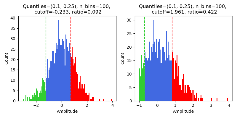
Here is shown the histogram of two units, with the vertical lines separating low- and high-amplitude regions.
On the left, we have a unit with no truncation at the left end, and the cutoff and ratio are small.
On the right, we have a unit with truncation at -1, and the cutoff and ratio are much larger.
Links to original implementations
From IBL implementation
Note: Compared to the original implementation, we have added a comparison between the low-amplitude bins to the largest bin (noise_ratio).
The selection of low-amplitude bins is based on the low_quantile rather than the number of bins.
Literature
Metric introduced by [IBL2024].