Benchmark module

Historically, this module was used to compare/benchmark sorters against ground truth With this, sorters can be challenge in multiple situations (noise, drift, small/high snr, small/high spike rate, high/small probe density, …).

The main idea is to generate a synthetic recording using the internal generators generate_drifting_recording() or external tools like *mearec. And then to compare the output of each sorter to the ground truth sorting. Then, theses comparisons can be plotted in various ways to explore all strengths and weakness of sorters tools. The very first paper of spikeinterface was about that, see [Buccino].

Since version, 0.102.0 the concept of benchmark has been extended to challenge/study specific steps of the sorting pipeline, for instance the motion estimation methods has been carrfully studied in [Garcia2024] or some localisation methods has been compared in [Scopin2024]. Also, very specific details (the ability for a sorting to recover collision spike) has been studied in [Garcia2022].

Now, almost all steps of the spike sorting step has implemented in spikeinterface and then all this steps can be benchmarked more or less the same way with dedicated classes:

• detect_peaks() methods can be compared with PeakDetectionStudy

• localize_peaks() methods can be compared with PeakLocalizationStudy

• estimate_motion() methods can be compared with MotionEstimationStudyStudy

• find_clusters_from_peaks() methods can be compared with ClusteringStudy

• find_spikes_from_templates() methods can be compared with MatchingStudy

And of course:

• run_sorter() with differents sorters (internal or external) can be compared with SorterStudy

All theses benchmark study classes share the same design :

• They accept as input a dict of “cases”. A case being a mix of one method (or one sorter) in a particular situation (drift or not, low/high snr, …) with some parameters. With this in mind, this is very easy to test either algorithm but also there parameters.

• Study classes has 4 steps : create cases, run methods, compute results and plot results.

• Study classes have dedicated plot functions or more general plotting (for instance accuracy vs snr)

• Study classes also cases handle the concept of “levels” : this allows you to compare several complexities at the same time. For instance, compare kilosort4 vs kilsort2.5 (level 0) for different noises amplitudes (level 1) combined with several motion vectors (level 2).

• When plotting levels can be grouped to make averages.

• Internally, they almost all use the comparison module. In short this module can compare a set of spiketrains against ground truth spiketrains. The van diagram (True Posistive, False positive, False negative) against each ground truth units is performed. An internal agreement matrix is also constructed. With this machinery many metrics can be taken to estimate the quality of a methods : accuracy, recall, precision

• Study classes are persistent on disk. The mechanism is based on an intrinsic organization into a “study_folder” with several subfolders: results, sorting_analyzer, run_logs, cases…

• By design a Study class has an associated Benchmark class to delegated the storage and the compute_result()

Example 1: compare some sorters : a ground truth study

The most high level class is to compare sorters against ground truth: SorterStudy()

Here a simple code block to generate

import spikeinterface as si
import spikeinterface.widgets as sw
from spikeinterface.benchmark import SorterStudy

# generate 2 simulated datasets (could be also mearec files)
rec0, gt_sorting0 = si.generate_ground_truth_recording(num_channels=4, durations=[30.], seed=2205)
rec1, gt_sorting1 = si.generate_ground_truth_recording(num_channels=4, durations=[30.], seed=91)

# step 1 : create cases and datasets
datasets = {
    "toy0": (rec0, gt_sorting0),
    "toy1": (rec1, gt_sorting1),
}

# define some "cases". Here we want to test tridesclous2 on 2 datasets and spykingcircus2 on one dataset
# so it is a two level study (sorter_name, dataset)
# this could be more complicated like (sorter_name, dataset, params)
cases = {
    ("tdc2", "toy0"): {
        "label": "tridesclous2 on tetrode0",
        "dataset": "toy0",
        "params": {"sorter_name": "tridesclous2"}
    },
    ("tdc2", "toy1"): {
        "label": "tridesclous2 on tetrode1",
        "dataset": "toy1",
        "params": {"sorter_name": "tridesclous2"}
    },
    ("sc2", "toy0"): {
        "label": "spykingcircus2 on tetrode0",
        "dataset": "toy0",
        "params": {
            "sorter_name": "spykingcircus2",
            "docker_image": True
        },
    },
}
# this initializes a folder
study_folder = "~/my_study_sorters"
study = SorterStudy.create(study_folder=study_folder, datasets=datasets, cases=cases,
                                levels=["sorter_name", "dataset"])

# Step 2 : run
# This internally does run_sorter() for all cases in one function
study.run()

# Step 3 : compute results
# Run the benchmark : this internally does compare_sorter_to_ground_truth() for all cases
study.compute_results()

# Step 4 : plots
study.plot_performances_vs_snr()
study.plot_performances_ordered()
study.plot_agreement_matrix()
study.plot_unit_counts()

# we can also go more internally and retrieve the comparison internal object like this
for case_key in study.cases:
    print('*' * 10)
    print(case_key)
    # raw counting of tp/fp/...
    comp = study.get_result(case_key)["gt_comparison"]
    # summary
    comp.print_summary()
    # some plots
    m = comp.get_confusion_matrix()
    w_comp = sw.plot_agreement_matrix(sorting_comparison=comp)

# We can also collect internal dataframes
# As shown previously, the performance is returned as a pandas dataframe.
# The spikeinterface.comparison.get_performance_by_unit() function
# gathers all the outputs in the study folder and merges them into a single dataframe.
# Same idea for spikeinterface.comparison.get_count_units()

# this is a dataframe
perfs = study.get_performance_by_unit()

# this is a dataframe
unit_counts = study.get_count_units()

# Study also has several plotting methods for plotting the result

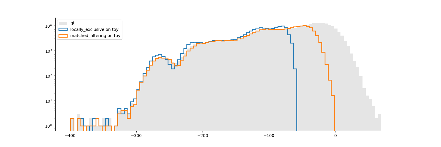
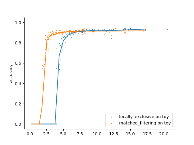
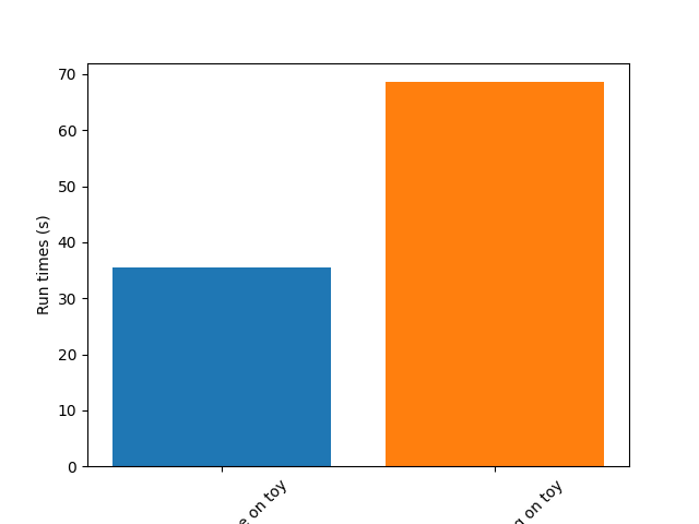
Example 2: compare peak detections

The detect_peaks() function propose mainly (with some variants) 2 main methods :

• “locally_exclussive” : a multichannel peak detection by threhold crossing that taken in account the neighbor channels

• “matched_filtering” : a method based on convolution by a kernel that “looks like a spike” at several spatial scales.

Here a very simple code to compare this 2 methods.

import spikeinterface.full as si
from spikeinterface.benchmark.benchmark_peak_detection import PeakDetectionStudy

si.set_global_job_kwargs(n_jobs=-1, progress_bar=True)

# generate
rec_static, rec_drifting, gt_sorting, extra_infos = si.generate_drifting_recording(
    probe_name="Neuropixels1-128",
    num_units=200,
    duration=300.,
    seed=2205,
    extra_outputs=True,
)

# small trick to get the ground truth peaks and max channels
extremum_channel_inds = dict(zip(gt_sorting.unit_ids, gt_sorting.get_property("max_channel_index")))
spikes = gt_sorting.to_spike_vector(extremum_channel_inds=extremum_channel_inds)
gt_peak = spikes

# step 1 : create dataset and cases dicts
datasets = {
    "data1": (rec_static, gt_sorting),
}

cases = {}
cases["locally_exclusive"] = {
    "label": "locally_exclusive on toy",
    "dataset": "data1",
    "init_kwargs": {"gt_peaks": gt_peak},
    "params": {
    "method": "locally_exclusive", "method_kwargs": {}},
}

# matched_filtering need a "waveform prototype"
ms_before, ms_after = 1.5, 2.5
from spikeinterface.sortingcomponents.tools import get_prototype_and_waveforms_from_recording
prototype, _, _ = get_prototype_and_waveforms_from_recording(rec_static, 5000, ms_before, ms_after)
cases["matched_filtering"] = {
    "label": "matched_filtering on toy",
    "dataset": "data1",
    "init_kwargs": {"gt_peaks": gt_peak},
    "params": {
    "method": "matched_filtering", "method_kwargs": {"prototype": prototype, "ms_before": ms_before}},
}

study_folder = "my_study_peak_detection"
study = PeakDetectionStudy.create(study_folder, datasets=datasets, cases=cases)
print(study)

# Step 2 : run
study.run()
# Step 3 : compute results
study.compute_analyzer_extension( {"templates":{}, "quality_metrics":{"metric_names": ["snr"]} } )
study.compute_results()
print(study)

# study can be re loaded
study_folder = "my_study_peak_detection"

study = PeakDetectionStudy(study_folder)

# Step 4 : plots
fig = study.plot_detected_amplitude_distributions()
fig = study.plot_performances_vs_snr(performance_names=["accuracy"])
fig = study.plot_run_times()

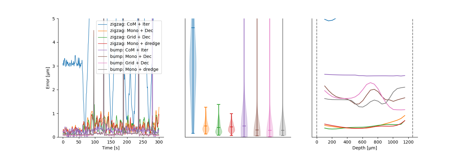
Example 3: compare motion estimation methods

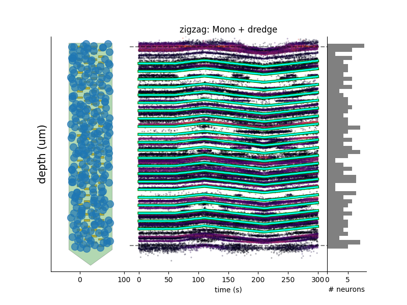
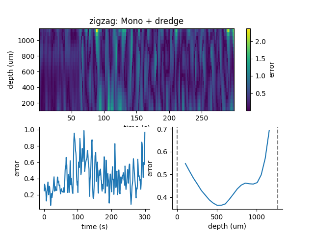
This paper [Garcia2024] was comparing sevral methods to estimate the motion in recordings. This was a proof of concept of the modularity and benchmarks in spikeinterface. In summary, motion estimation is done in 3 steps : detect peaks, localize peaks and motion inference. For theses steps there are sevral possible methods, so combining and comparing performance was the main topic of this niche paper.

This paper was using on the mearec package for generation and a previous version of spikeinterface for benchmark but re-generating the same figures should be pretty easy in the new version of spikeinterface.

Note that since this puplication, new methods has been published (DREDGe and MEDiCINe) and implemented in spikeinterface so runnning a new comparison could make sens.

Lets be open-and-reproducible-science, this is so trendy. This 120 lines script will make the same job done [Garcia2024].

# If a random reader reach this line of documentation, I hope that this reader will be impressed by the
# quality of method implementation but also by the smart design of the benchmark framework!
# In any case, this reader be must be a very spike sorting fanatic person or insomniac.

import spikeinterface.full as si
from spikeinterface.benchmark.benchmark_motion_estimation import MotionEstimationStudy

si.set_global_job_kwargs(n_jobs=0.8, chunk_duration="1s")

probe_name = 'Neuropixels1-128':
num_units = 250

datasets = {}
drift_info = {}
static, drifting, sorting, info = si.generate_drifting_recording(
    num_units=num_units,
    duration=300.,
    probe_name=probe_name,
    generate_sorting_kwargs=dict(
        firing_rates=(2.0, 8.0),
        refractory_period_ms=4.0
    ),
    generate_displacement_vector_kwargs=dict(
        displacement_sampling_frequency=5.0,
        drift_start_um=[0, 20],
        drift_stop_um=[0, -20],
        drift_step_um=1,
        motion_list=[
            dict(
                drift_mode="zigzag",
                non_rigid_gradient=None,
                t_start_drift=60.0,
                t_end_drift=None,
                period_s=200,
            ),
        ],
    ),
    extra_outputs=True,
    seed=2205,
)
datasets["zigzag"] = (drifting, sorting)
drift_info["zigzag"]  = info


static, drifting, sorting, info = si.generate_drifting_recording(
    num_units=num_units,
    duration=300.,
    probe_name=probe_name,
    generate_sorting_kwargs=dict(
        firing_rates=(2.0, 8.0),
        refractory_period_ms=4.0
    ),
    generate_displacement_vector_kwargs=dict(
        displacement_sampling_frequency=5.0,
        drift_start_um=[0, 20],
        drift_stop_um=[0, -20],
        drift_step_um=1,
        motion_list=[
            dict(
                drift_mode="bump",
                non_rigid_gradient=None,
                t_start_drift=60.0,
                t_end_drift=None,
                bump_interval_s=(30, 80.),
            ),
        ],
    ),
    extra_outputs=True,
    seed=2205,
)
datasets["bump"] = (drifting, sorting)
drift_info["bump"]  = info

cases = {}
for dataset_name in datasets:
    for method_label, loc_method, est_method in [
        ("CoM + Iter", "center_of_mass", "iterative_template"),
        ("Mono + Dec", "monopolar_triangulation", "decentralized"),
        ("Grid + Dec", "grid_convolution", "decentralized"),
        ("Mono + dredge", "monopolar_triangulation", "dredge_ap"),

    ]:
        label = f"{dataset_name}: {method_label}"
        key = (dataset_name, method_label)

        estimate_motion_kwargs=dict(
            method=est_method,
            bin_s=1.0,
            bin_um=5.0,
            rigid=False,
            win_step_um=50.0,
            win_scale_um=200.0,
        )

        cases[key] = dict(
            label=label,
            dataset=dataset_name,
            init_kwargs=dict(
                unit_locations=drift_info[dataset_name]["unit_locations"],
                # displacement on Y
                unit_displacements=drift_info[dataset_name]["unit_displacements"],
                displacement_sampling_frequency=drift_info[dataset_name]["displacement_sampling_frequency"],
                direction="y",
            ),
            params=dict(
                detect_kwargs=dict(method="locally_exclusive", detect_threshold=7.0),
                select_kwargs=None,
                localize_kwargs=dict(method=loc_method),
                estimate_motion_kwargs=estimate_motion_kwargs,
            ),
        )

study = MotionEstimationStudy(study_folder)
study.run(verbose=True)
study.compute_results()

study.plot_summary_errors()
study.plot_drift(raster=True, case_keys=[('zigzag', 'Mono + dredge')])
study.plot_errors(case_keys=[('zigzag', 'Mono + dredge')])

Other examples

With some imagination and by exploring a bit this repo, testing new methods for spike sorting steps is now an easy task : clustering, template matching, motion estimation, peak detection, …